JPMorgan Chase & Co. Quantitative Research Virtual Experience Program

Task 1

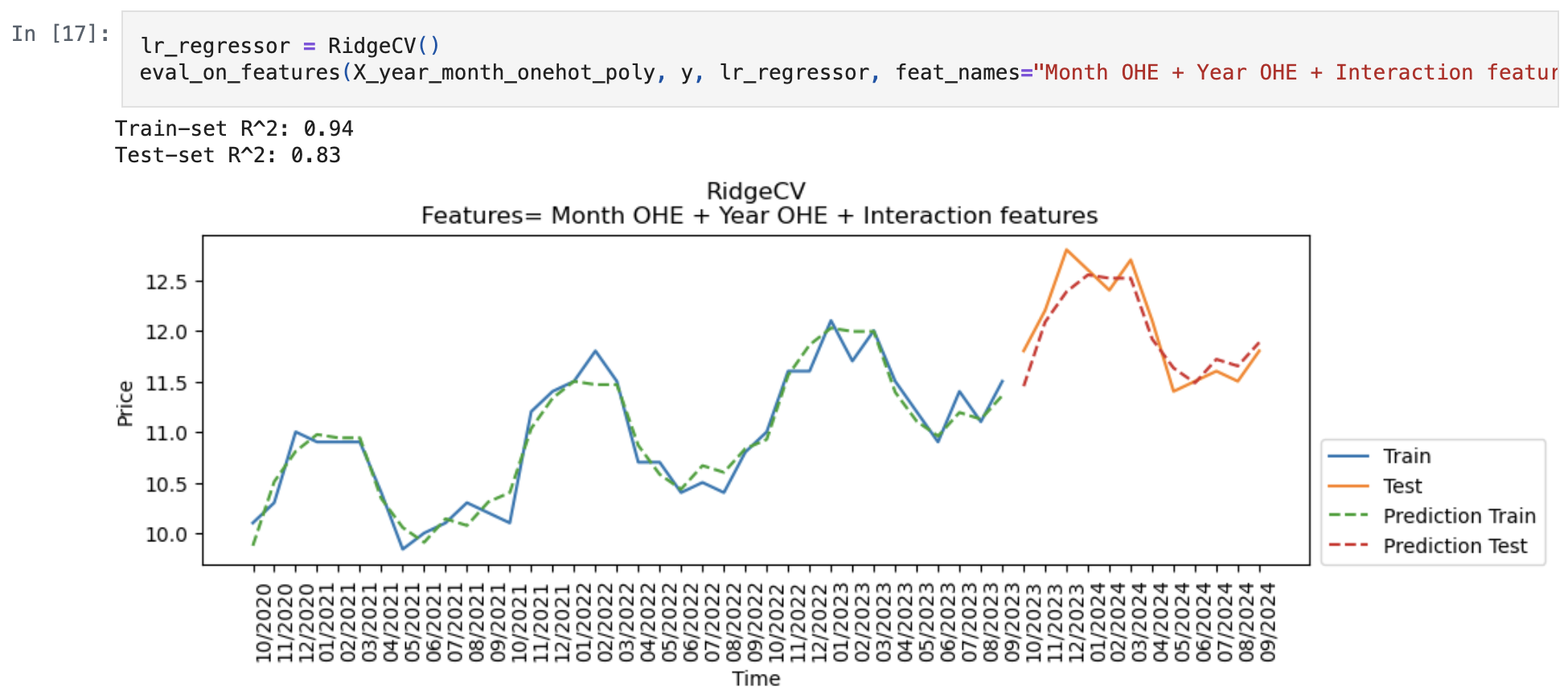
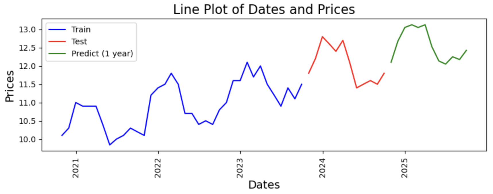
• Tested various methods to encode time, such as POSIX time, month and year features and one-hot encoding (OHE) of months and years, along with implementing interaction features and lag features, for the time series analysis of price data, by plotting out their prediction and calculating their \(R^{2}\) score for both the train and test data.
• Utilised a linear model lr_regressor_nolag() that uses one-hot encoding for months and years along with interaction features to predict future price data, under the assumption that price will increase indefinitely over the years, and will have the same pattern of price changes across months.

lr_regressor_nolag

Line Plot of Dates and Prices

Task 2

• Create a prototype pricing model that can go through further validation and testing before being put into production.
• Inputs
  • Dictionary of injection and withdrawal dates (in the form %Y-%m-%d) and amounts
  • List of prices at which the commodity can be purchased/sold on those dates
  • Rate at which the gas can be injected/withdrawn
  • Maximum volume that can be stored
  • Fixed fees per month for storing
• Output: Predicted contract price

```{python}
def contractprice(injewithdates, pricelist, gasrate, maxvol, storagecost):
    """
    Given existing price data and input parameters, produce contract price. 
    Assumes that injection and withdrawal involve buying and selling of fuel respectively.
    
    Parameters:
    -----------
        
    injewithdates: dictionary
        Dictionary of injection and withdrawal dates (in the form %Y-%m-%d) and amounts.
        Injections are positive, withdrawals are negative.
        
    pricelist: dataframe 
        Prices at which the commodity can be purchased/sold on those dates.

    gasrate: float 
        Rate at which the gas can be injected/withdrawn.
        
    maxvol: float 
        Maximum volume that can be stored.
        
    storagecost: float
        Fixed fees per month for storing.

    Returns:
    --------
    Contract price. 
    """ 

    amount = 0
    dict1 = {pd.to_datetime(key): value for key, value in injewithdates.items()}
    dict2 = pricelist.to_dict()["Prices"]
    sumcosts = {key: None for key in dict1.keys()}
    for k, v in dict1.items(): 
        if (v < 0) and (amount >= abs(v)): 
            amount -= v
        elif ((amount + v) <= maxvol): 
            amount += v
        else: 
            raise Exception("Invalid storage amount")
        
        if k in df_exist_dict: 
            sumcosts[k] = v * dict2[k]
        else: 
            sumcosts[k] = v * pricepredict([k])["Prices"][0]

    display(sumcosts)
    finalexchanges = sum(sumcosts.values())
    date1 = min(dict1.keys())
    date2 = max(dict1.keys())
    nummonths = 12 * relativedelta(date2, date1).years + relativedelta(date2, date1).months
    
    totalgasprice = gasrate * sum(abs(number) for number in dict1.values())
    total_storagecost = storagecost * nummonths
    
    final_price = finalexchanges - totalgasprice - total_storagecost
    return final_price
```

Task 3

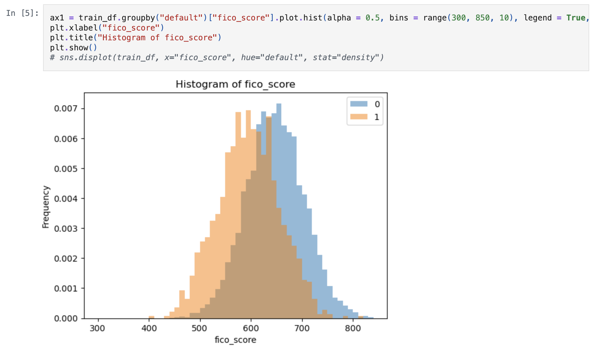
• Assessed a right-censored loan book using survival analysis models (e.g. Kaplan-Meier Survival Curve) to estimate a customer’s probability of default, and by proxy the expected loss
• Equation: \(EL = PD * (1 - RR) * EAD\)
  • \(EL\) = Expected loss
  • \(PD\) = Probability of default (KM_estimate)
  • \(RR\) = Recovery rate (Provided as 10%)
  • \(EAD\) = Exposure at default (Due to lack of provided information, assume this is total_debt_outstanding)

```{python}
kmf = lifelines.KaplanMeierFitter()
kmf.fit(train_df_surv["years_employed"], train_df_surv["default"]);
pdestimates = kmf.survival_function_.to_dict()["KM_estimate"]

def expectedloss(total_debt_outstanding, years_employed, recovery_rate = 0.1, default = 0, survival_estimates = pdestimates): 
    """
    Returns expected losses given loan properties. 
    
    Parameters:
    -----------
        
    total_debt_outstanding: float
        Total outstanding debt. 

    years_employed: int
        Number of years individual has been employed. 

    recovery_rate: float
        Amount recovered when a loan defaults.

    default: bool
        Whether or not the individual has defaulted by this point or not. 
        Already defaulted individuals will assume probability of 1, non-defaulted individuals will assume survival_estimates.

    survival_estimates: dictionary 
        Dictionary of survival probabilities corresponding to the number of years individual has been employed.
        
    Returns:
    --------
    Corresponding expected loss given 
    """ 
    km_estimate = 1 
    if default == 0: 
        km_estimate = survival_estimates.get(years_employed)
    expected_loss = km_estimate * (1 - recovery_rate) * total_debt_outstanding
    return expected_loss 
```

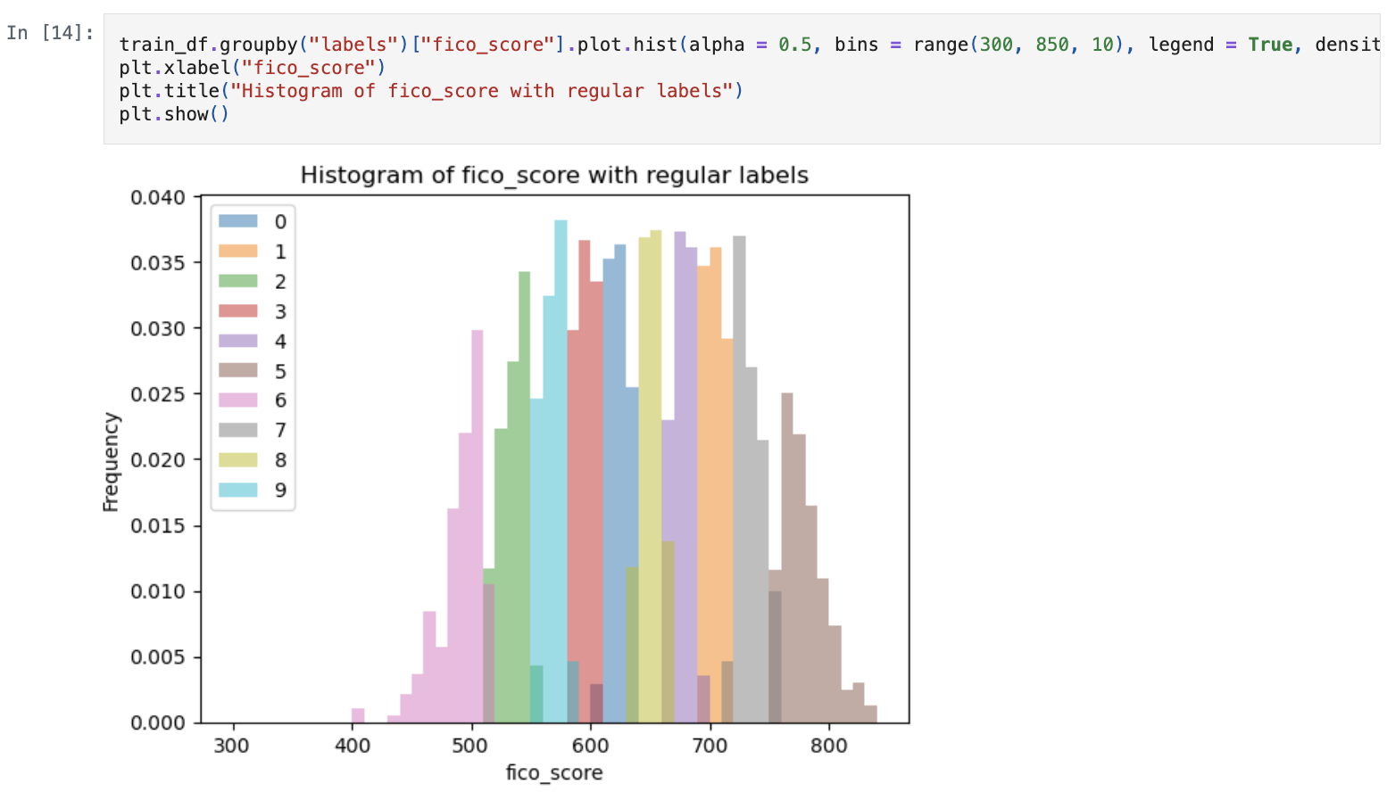
Task 4

• Utilised dynamic programming to convert FICO scores into categorical data to predict defaults

FICO distributions

• Options considered:
  • Use mean and standard distribution as intervals for data.
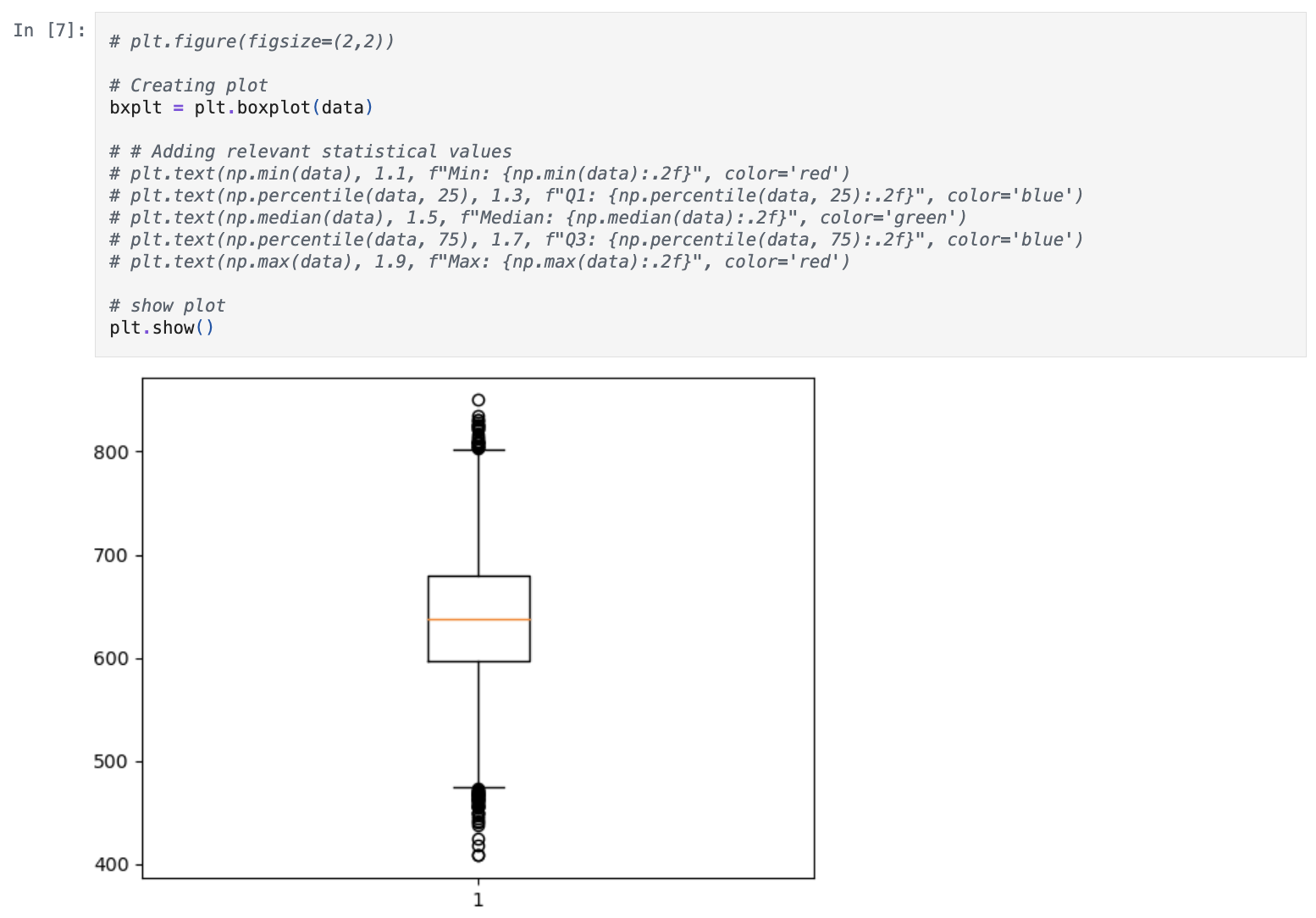
  • Use quartiles and boxplot whiskers.
  • KMeans to create intervals.

Mean and Standard Distribution

Boxplot

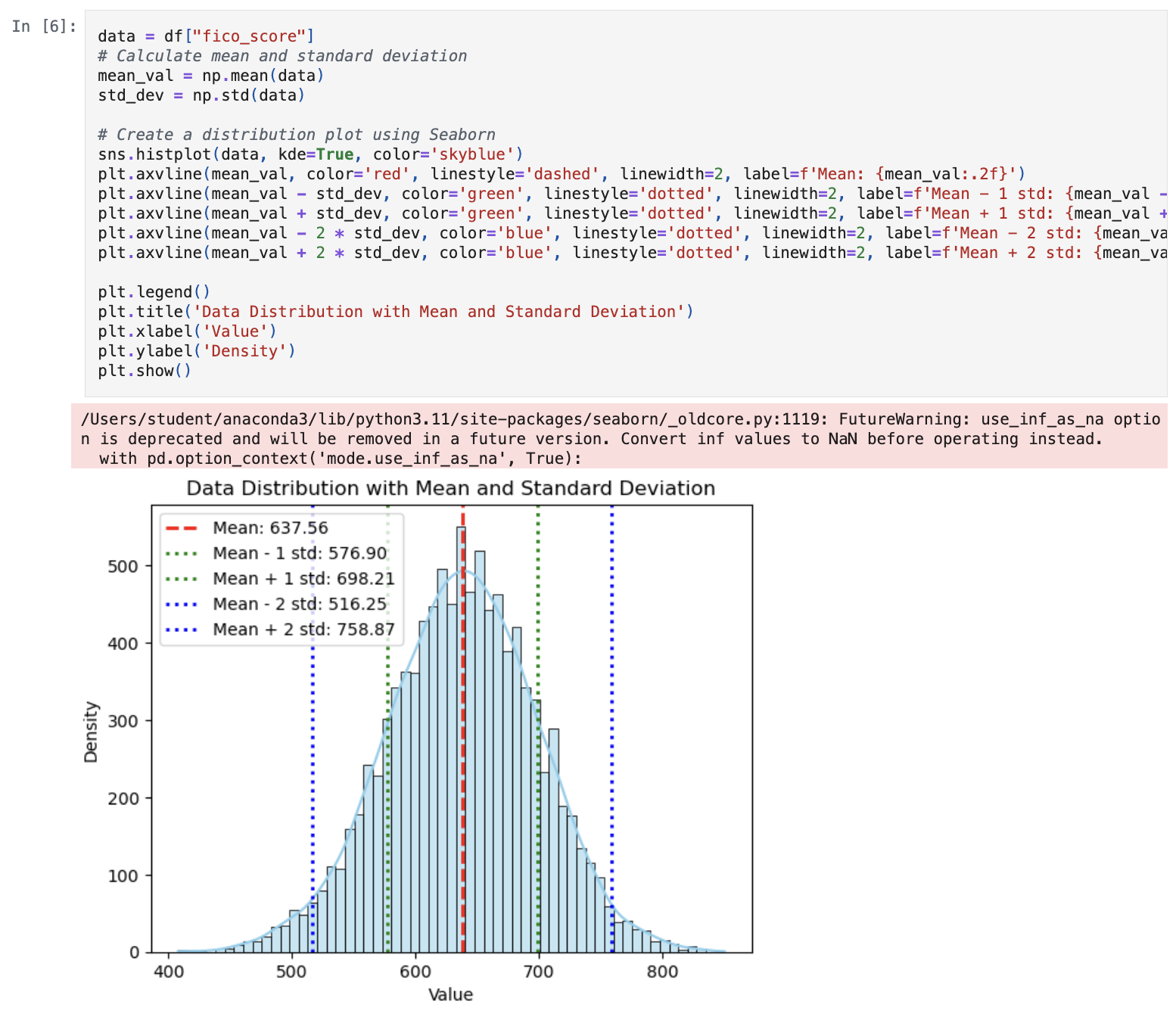
• KMeans was selected due to allowing any number of buckets to be created by the user’s choosing.
  • None of the labels overlap in terms of specific values.
  • Provided example uses 10 buckets

FICO Labelling